3. 机器学习中为什么需要梯度下降_【干货】机器学习 | 为什么机器能“学习”？——感知器和梯度下降...

大家好我是梁力天，今天我来给大家整理一下感知器 (perceptron model) 和梯度下降算法 (gradient descent) 的知识。

source: https://cs.stanford.edu/

An intuitive understanding of perceptron

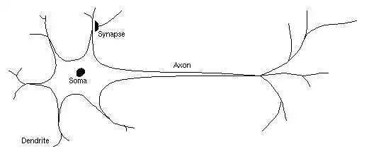
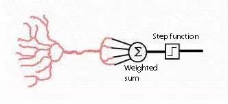
感知器是一种简单的线性分类器，但感知器解决分类问题的思路不同于贝叶斯，决策树等模型。感知器模仿了人类神经元电信号传递数据的方式，感知器用参数 ( θ ) 对特征 ( x ) 点乘得到类似于输入数据的总信号强度 ( θx^T )。因为感知器内部的参数 ( θ ) 随着学习在不断改变，所以对不同特征的输入信号组合会有不同的反应。总信号强度通过激活函数 (activation function) ，得到这个感知器(神经元)的输出(电)信号大小 ( σ(θx^T) )。以判断是否有感受。

举一个不严谨的例子：

比如下图为例，假设这个感知器的放电代表你想吃冰激凌。那么输入信号可以是：天气温度 ( x₁ )，身体内当前糖分 ( x₂ )，看到冰激凌广告 ( x₃ ) 等。如果天气温度很高 35 度 ( x₁=35 )，目前糖分 30% ( x₂=0.3 )，恰好你看电视上正在播一个冰激凌的广告 1 ( x₃=1 )，这个神经元就会被激活 ( x=[35,0.3,1],y=1 )。带动其他神经元放电，最后感受到想吃冰激凌。如果当前温度 2 度, 糖分95%, 而且没有看到冰激凌广告 0，这个感知器就不会放电，也就是不想吃冰激凌 ( x=[2,0.95,0],y=0 )。

这种情况下，这个感知器就是 “是否想吃冰激凌” 的分类器，0 为不想吃，1 为想吃。

一个刚出生的婴儿，并不会做什么，因为他所有神经元内的参数是随机的。但是经过训练，婴儿也能有很灵敏的感受，比如冷了，热了，想吃饭等等。等长大了，就可以理解为一部分神经元的参数经过训练已经收敛至local minimum，就可以做出想吃冰激凌等等的判断。

想要得到正确的感知/分类结果，感知器通过学习算法，不断调整内部参数 (θ) 逐渐接近正确的分类结果。调整参数的方式和人类学习是一样的。感知器对每一个数据点尝试得出一个不一定正确结果，使用cost function和正确结果比较差了多少，然后向接近正确结果的方向更改参数(cost function 对参数的逆梯度方向)。这样就能逐渐提高模型分类正确率。这种优化算法 (optimization algorithm) 有很多，比如Adam, rmsprop, Adagrad等，今天我就就使用最简单的随机梯度下降 (Stochastic Gradient Descent / SGD) 算法优化这个感知器。

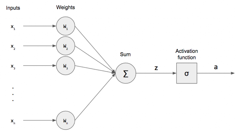
现在让我们来深入了解一下感知器的组成部分

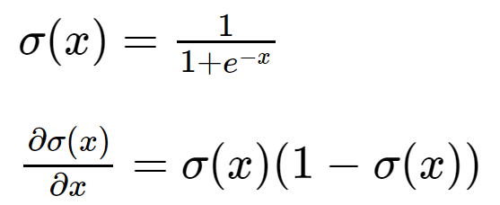
import numpy as npimport matplotlib.pyplot as plt

Defining our perceptron Activation function and its derivative (in this case: sigmoid)

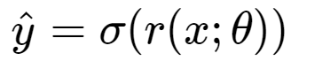
在这种情况下，如果 linear response r(x;θ)=θx^T 是 2.5，即σ(r(x))>0.5，分类结果即为 class 1，如果σ(r(x))<0.5，分类结果为0

def sigmoid(x):    ''' sigmoid activation function '''    return 1 / (1 + np.exp(-x))def dsigmoid(x):    return sigmoid(x) * (1 - sigmoid(x))x = np.linspace(-10,10,100)plt.plot(x, sigmoid(x)); plt.show()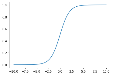

Loss function and its derivative (ex: mean squared error)

今天我使用均方误差测量函数测量误差大小，不过任何可导误差测量函数都可以，比如negative log liklihood，或categorical cross entropy(需要计算梯度进行优化，所以需要可导函数)

def mse(y, yhat):    ''' mean squared error '''    dy = y - yhat    return dy.dot(dy)def dmse(y, yhat):    return -2 * (y - yhat)

在我们看感知器的定义class之前，我们先看一下几个核心算法

1. 如何计算 linear response

2. 如何计算 forward pass，即分类器的分类结果

3. 如何推导梯度下降计算模型更新大小，即训练算法，并且适用于所有activation function 和 loss function

1. Calculating the linear response

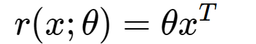
def r(self, x):    ''' calculate linear response '''    thetaxT = self.theta.dot(np.concatenate(([1], x)))    # concatenate 1 in-front of x to calculate bias    return thetaxT

2. Calculate forward pass (prediction result)

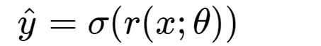
def forward(self, x):    ''' calculate prediction '''    yhat = self.activation(self.r(x))    return yhat

3. Derive the gradient descent algorithm

We know that  yHat  is calculated as:

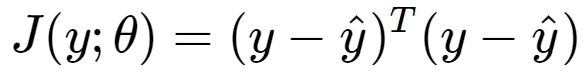
We know that loss is defined as:

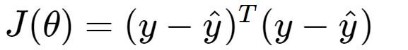
We need to update our model using stochastic gradient descent SGD(learning_rate=alpha):

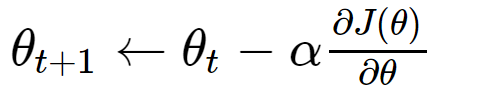
in pseudocode:

theta = theta - lr * gradient

which is updating the parameter towards the negative direction of the current gradient of loss function multiplied by learning rate alpha

the only term that we need to calculate is the gradient of J(θ) with respect to θ which is:  ∂J(θ)/∂θ

to calculate the gradient, and generalize to all activation/loss functions, we can use the chain rule of derivative:

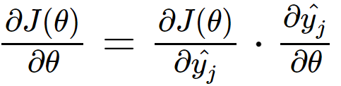
by applying chain rule on the partial derivative of  yHat  with respect to  θ , we get:

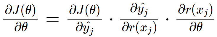
where the first term is the gradient of loss function with respect to prediction result

the second term is the gradient of prediction result with respect to the linear response

the third term is the gradient of linear response with respect to the parameters, which is equal to  X_j , then we can get

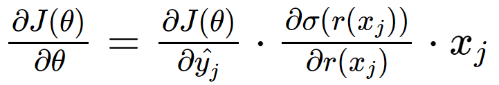
in pseudocode:

gradient = dloss(y, yhat) * dactivation(r(xj)) * xj

now we know how to calculate gradient, lets jump into the code of stochastic gradient descent algorithm

def backprop(self, X, Y, lr=1e-5, batch_size=1, epochs=1, verbose=0, frequency=1):        ''' stochastic gradient descent '''        currentfrequency = frequency                 # go through our dataset {epochs} times        for epoch in range(epochs):                        # calculate gradient update for each data point            for x, y in zip(X,Y):                                # calculate prediction                yhat = self.forward(x)                                # calculate gradient                gradient = self.dlossfunc(y, yhat)       # dJ(theta)/dtheta                           * self.dactivation(self.r(x)) # dsimoid(r(x))/dr(x)                           * np.concatenate(([1], x))    # x                                # taking a step toward negative gradient                self.theta = self.theta - lr * gradient                        # if verbosity is required, plot the current decision boundary            if verbose > 0 and currentfrequency==0:                plt.scatter(X[:,0], X[:,1], c=Y)                plt.title(f'epoch {epoch} acc={self.acc(X, Y)}')                self.plot_boundary(-2, 2)                plt.axis('equal')                plt.show()                currentfrequency = frequency                        else:                currentfrequency -= 1

将上述的所有步骤合并，我们就得到了一个可以学习的感知器

class Perceptron:        def __init__(self, input_shape: int, activation=sigmoid, lossfunc=mse, dactivation=dsigmoid, dlossfunc=dmse):        ''' initialize weight vector w '''        # parameter dimension        self.d = input_shape         # 1 extra weight for bias        self.theta = np.random.rand(input_shape + 1) - 0.5                # storing the activation and loss function        self.activation = activation        self.dactivation = dactivation        self.lossfunc = lossfunc        self.dlossfunc = dlossfunc            def plot_boundary(self, horizontalx, horizontaly):        x=np.linspace(horizontalx, horizontaly, 100)        plt.plot(x, -self.theta[0] / self.theta[2] + x * -self.theta[1] / self.theta[2])        plt.axis('equal')            def r(self, x):        ''' calculate linear response '''        thetaxT = self.theta.dot(np.concatenate(([1], x)))        return thetaxT    def forward(self, x):        ''' calculate prediction '''        yhat = self.activation(self.r(x))        return yhat        def acc(self, X, Y):        return np.sum(np.array(np.apply_along_axis(arr=X, func1d=lambda x: self.forward(x), axis=1) > 0.5, dtype='int') == Y) / Y.shape[0]        def backprop(self, X, Y, lr=1e-5, batch_size=1, epochs=1, verbose=0, frequency=1):        ''' stochastic gradient descent '''        currentfrequency = frequency                for epoch in range(epochs):            for x, y in zip(X,Y):                                # calculate prediction                yhat = self.forward(x)                                # calculate gradient                #print(gradient)                gradient = self.dlossfunc(y, yhat)  * self.dactivation(self.r(x)) * np.concatenate(([1], x))                                # gradient descent                #print(gradient)                #print(self.theta)                self.theta = self.theta - lr * gradient                        # if verbosity is required, plot the current decision boundary            if verbose > 0 and currentfrequency==0:                plt.scatter(X[:,0], X[:,1], c=Y)                plt.title(f'epoch {epoch} acc={self.acc(X, Y)}')                self.plot_boundary(-2, 2)                plt.axis('equal')                plt.show()                currentfrequency = frequency                        else:                currentfrequency -= 1

让我们简单的测试一下模型的表现情况，为了实验的可重复性，我将三个随机的初始参数hard code进了模型参数。

model = Perceptron(input_shape=2)model.theta = np.array([-0.45531969, -0.49536212,  0.48505017])print(f'theta={model.theta}')

theta=[-0.45531969 -0.49536212  0.48505017]

我们使用 or 门作为训练数据，可以看出，现在模型是不能够正确分类紫色(class 0)和黄色 (class 1) 的

X = np.array([[1,1],[-1,1],[-1,-1],[1,-1]])Y = np.array([1,1,0,1])plt.scatter(X[:,0], X[:,1], c=Y)model.plot_boundary(-2,2)plt.show()

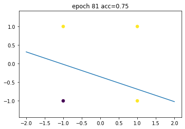
现在，我们用梯度下降开始训练这个感知器

model.backprop(X, Y, lr=2e-2, epochs=200, verbose=1, frequency=40)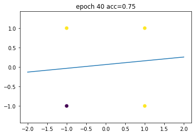

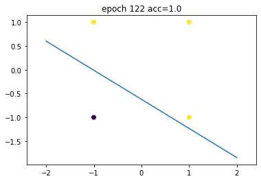
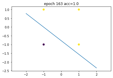
model.acc(X, Y)

1.0

终于，在遍历这个数据集163次之后 (163 epochs)，loss converged，我们得到了一个可以正确分类所有数据的感知器。

感知器是一种非常强大的分类方式，虽然训练的速度不快，但是训练结束后，分类的时间复杂度非常低，而且结果非常准确。当然，这只是一个线性分类器，但真实世界中的数据集会更加复杂，有更复杂的分类边界 (decision boundary)。并且根据人类大脑的神经结构，人们设计了一种现在非常流行的机器学习模型：神经网络。而神经网络的building block，就是感知器。神经网络就是多个感知器用不同的方法连接在一起，如果你喜欢我讲解机器学习算法的方式，请关注CUCS，下期推文，我们一起来了解一下神经网络。

文案 / CUCS学术部 梁力天

编辑 / CUCS宣传部

© CUCS 2020.11