作者 |?李秋鍵
責編 | Carol
封圖 |?CSDN?付費下載自視覺中國
近幾年來語音識別技術得到了迅速發展,從手機中的Siri語音智能助手、微軟的小娜以及各種平臺的智能音箱等等,各種語音識別的項目得到了廣泛應用。
語音識別屬于感知智能,而讓機器從簡單的識別語音到理解語音,則上升到了認知智能層面,機器的自然語言理解能力如何,也成為了其是否有智慧的標志,而自然語言理解正是目前難點。
波速球半球訓練動作。同時考慮到目前大多數的語音識別平臺都是借助于智能云,對于語音識別的訓練對于大多數人而言還較為神秘,故今天我們將利用python搭建自己的語音識別系統。
最終模型的識別效果如下:
實驗前的準備
首先我們使用的python版本是3.6.5所用到的庫有cv2庫用來圖像處理;
Numpy庫用來矩陣運算;Keras框架用來訓練和加載模型。Librosa和python_speech_features庫用于提取音頻特征。Glob和pickle庫用來讀取本地數據集。
波巴士訓練、首先數據集使用的是清華大學的thchs30中文數據。
這些錄音根據其文本內容分成了四部分,A(句子的ID是1~250),B(句子的ID是251~500),C(501~750),D(751~1000)。ABC三組包括30個人的10893句發音,用來做訓練,D包括10個人的2496句發音,用來做測試。
data文件夾中包含(.wav文件和.trn文件;trn文件里存放的是.wav文件的文字描述:第一行為詞,第二行為拼音,第三行為音素);
數據集如下:
紋波?首先人的聲音是通過聲道產生的,聲道的形狀決定了發出怎樣的聲音。如果我們可以準確的知道這個形狀,那么我們就可以對產生的音素進行準確的描述。聲道的形狀在語音短時功率譜的包絡中顯示出來。而MFCCs就是一種準確描述這個包絡的一種特征。
其中提取的MFCC特征如下圖可見。
?
故我們在讀取數據集的基礎上,要將其語音特征提取存儲以方便加載入神經網絡進行訓練。
a波增強訓練費用多少。其對應的代碼如下:
#讀取數據集文件
text_paths?=?glob.glob('data/*.trn')
total?=?len(text_paths)
print(total)
with?open(text_paths[0],?'r',?encoding='utf8')?as?fr:lines?=?fr.readlines()
print(lines)
#數據集文件trn內容讀取保存到數組中
texts?=?[]
paths?=?[]
for?path?in?text_paths:with?open(path,?'r',?encoding='utf8')?as?fr:lines?=?fr.readlines()line?=?lines[0].strip('\n').replace('?',?'')texts.append(line)paths.append(path.rstrip('.trn'))
print(paths[0],?texts[0])
#定義mfcc數
mfcc_dim?=?13#根據數據集標定的音素讀入
def?load_and_trim(path):audio,?sr?=?librosa.load(path)energy?=?librosa.feature.rmse(audio)frames?=?np.nonzero(energy?>=?np.max(energy)?/?5)indices?=?librosa.core.frames_to_samples(frames)[1]audio?=?audio[indices[0]:indices[-1]]?if?indices.size?else?audio[0:0]
return?audio,?sr
#提取音頻特征并存儲
features?=?[]
for?i?in?tqdm(range(total)):path?=?paths[i]audio,?sr?=?load_and_trim(path)features.append(mfcc(audio,?sr,?numcep=mfcc_dim,?nfft=551))
print(len(features),?features[0].shape)
在進行神經網絡加載訓練前,我們需要對讀取的MFCC特征進行歸一化,主要目的是為了加快收斂,提高效果和減少干擾。然后處理好數據集和標簽定義輸入和輸出即可。
對應代碼如下:
#隨機選擇100個數據集
samples?=?random.sample(features,?100)
samples?=?np.vstack(samples)
#平均MFCC的值為了歸一化處理
mfcc_mean?=?np.mean(samples,?axis=0)
#計算標準差為了歸一化
mfcc_std?=?np.std(samples,?axis=0)
print(mfcc_mean)
print(mfcc_std)
#歸一化特征
features?=?[(feature?-?mfcc_mean)?/?(mfcc_std?+?1e-14)?for?feature?in?features]
#將數據集讀入的標簽和對應id存儲列表
chars?=?{}
for?text?in?texts:for?c?in?text:chars[c]?=?chars.get(c,?0)?+?1
chars?=?sorted(chars.items(),?key=lambda?x:?x[1],?reverse=True)
chars?=?[char[0]?for?char?in?chars]
print(len(chars),?chars[:100])
char2id?=?{c:?i?for?i,?c?in?enumerate(chars)}
id2char?=?{i:?c?for?i,?c?in?enumerate(chars)}
data_index?=?np.arange(total)
np.random.shuffle(data_index)
train_size?=?int(0.9?*?total)
test_size?=?total?-?train_size
train_index?=?data_index[:train_size]
test_index?=?data_index[train_size:]
#神經網絡輸入和輸出X,Y的讀入數據集特征
X_train?=?[features[i]?for?i?in?train_index]
Y_train?=?[texts[i]?for?i?in?train_index]
X_test?=?[features[i]?for?i?in?test_index]
Y_test?=?[texts[i]?for?i?in?test_index]
其中包括訓練的批次,卷積層函數、標準化函數、激活層函數等等。
穩中二波、其中第?個維度為??段的個數,原始語?越長,第?個維度也越?,?第?個維度為 MFCC 特征的維度。得到原始語?的數值表?后,就可以使? WaveNet 實現。由于 MFCC 特征為?維序列,所以使? Conv1D 進?卷積。?因果是指,卷積的輸出只和當前位置之前的輸?有關,即不使?未來的?特征,可以理解為將卷積的位置向前偏移。WaveNet 模型結構如下所?:
具體如下可見:
batch_size?=?16
#定義訓練批次的產生,一次訓練16個
def?batch_generator(x,?y,?batch_size=batch_size):offset?=?0while?True:offset?+=?batch_sizeif?offset?==?batch_size?or?offset?>=?len(x):data_index?=?np.arange(len(x))np.random.shuffle(data_index)x?=?[x[i]?for?i?in?data_index]y?=?[y[i]?for?i?in?data_index]offset?=?batch_sizeX_data?=?x[offset?-?batch_size:?offset]Y_data?=?y[offset?-?batch_size:?offset]X_maxlen?=?max([X_data[i].shape[0]?for?i?in?range(batch_size)])Y_maxlen?=?max([len(Y_data[i])?for?i?in?range(batch_size)])X_batch?=?np.zeros([batch_size,?X_maxlen,?mfcc_dim])Y_batch?=?np.ones([batch_size,?Y_maxlen])?*?len(char2id)X_length?=?np.zeros([batch_size,?1],?dtype='int32')Y_length?=?np.zeros([batch_size,?1],?dtype='int32')for?i?in?range(batch_size):X_length[i,?0]?=?X_data[i].shape[0]X_batch[i,?:X_length[i,?0],?:]?=?X_data[i]Y_length[i,?0]?=?len(Y_data[i])Y_batch[i,?:Y_length[i,?0]]?=?[char2id[c]?for?c?in?Y_data[i]]inputs?=?{'X':?X_batch,?'Y':?Y_batch,?'X_length':?X_length,?'Y_length':?Y_length}outputs?=?{'ctc':?np.zeros([batch_size])}
epochs?=?50
num_blocks?=?3
filters?=?128
X?=?Input(shape=(None,?mfcc_dim,),?dtype='float32',?name='X')
Y?=?Input(shape=(None,),?dtype='float32',?name='Y')
X_length?=?Input(shape=(1,),?dtype='int32',?name='X_length')
Y_length?=?Input(shape=(1,),?dtype='int32',?name='Y_length')
#卷積1層
def?conv1d(inputs,?filters,?kernel_size,?dilation_rate):return?Conv1D(filters=filters,?kernel_size=kernel_size,?strides=1,?padding='causal',?activation=None,dilation_rate=dilation_rate)(inputs)
#標準化函數
def?batchnorm(inputs):return?BatchNormalization()(inputs)
#激活層函數
def?activation(inputs,?activation):return?Activation(activation)(inputs)
#全連接層函數
def?res_block(inputs,?filters,?kernel_size,?dilation_rate):hf?=?activation(batchnorm(conv1d(inputs,?filters,?kernel_size,?dilation_rate)),?'tanh')hg?=?activation(batchnorm(conv1d(inputs,?filters,?kernel_size,?dilation_rate)),?'sigmoid')h0?=?Multiply()([hf,?hg])ha?=?activation(batchnorm(conv1d(h0,?filters,?1,?1)),?'tanh')hs?=?activation(batchnorm(conv1d(h0,?filters,?1,?1)),?'tanh')return?Add()([ha,?inputs]),?hs
h0?=?activation(batchnorm(conv1d(X,?filters,?1,?1)),?'tanh')
shortcut?=?[]
for?i?in?range(num_blocks):for?r?in?[1,?2,?4,?8,?16]:h0,?s?=?res_block(h0,?filters,?7,?r)shortcut.append(s)
h1?=?activation(Add()(shortcut),?'relu')
h1?=?activation(batchnorm(conv1d(h1,?filters,?1,?1)),?'relu')
#softmax損失函數輸出結果
Y_pred?=?activation(batchnorm(conv1d(h1,?len(char2id)?+?1,?1,?1)),?'softmax')
sub_model?=?Model(inputs=X,?outputs=Y_pred)#計算損失函數
def?calc_ctc_loss(args):y,?yp,?ypl,?yl?=?args
return?K.ctc_batch_cost(y,?yp,?ypl,?yl)
訓練的過程如下可見:
ctc_loss?=?Lambda(calc_ctc_loss,?output_shape=(1,),?name='ctc')([Y,?Y_pred,?X_length,?Y_length])
#加載模型訓練
model?=?Model(inputs=[X,?Y,?X_length,?Y_length],?outputs=ctc_loss)
#建立優化器
optimizer?=?SGD(lr=0.02,?momentum=0.9,?nesterov=True,?clipnorm=5)
#激活模型開始計算
model.compile(loss={'ctc':?lambda?ctc_true,?ctc_pred:?ctc_pred},?optimizer=optimizer)
checkpointer?=?ModelCheckpoint(filepath='asr.h5',?verbose=0)
lr_decay?=?ReduceLROnPlateau(monitor='loss',?factor=0.2,?patience=1,?min_lr=0.000)
#開始訓練
history?=?model.fit_generator(generator=batch_generator(X_train,?Y_train),steps_per_epoch=len(X_train)?//?batch_size,epochs=epochs,validation_data=batch_generator(X_test,?Y_test),validation_steps=len(X_test)?//?batch_size,callbacks=[checkpointer,?lr_decay])
#保存模型
sub_model.save('asr.h5')
#將字保存在pl=pkl中
with?open('dictionary.pkl',?'wb')?as?fw:pickle.dump([char2id,?id2char,?mfcc_mean,?mfcc_std],?fw)
train_loss?=?history.history['loss']
valid_loss?=?history.history['val_loss']
plt.plot(np.linspace(1,?epochs,?epochs),?train_loss,?label='train')
plt.plot(np.linspace(1,?epochs,?epochs),?valid_loss,?label='valid')
plt.legend(loc='upper?right')
plt.xlabel('Epoch')
plt.ylabel('Loss')
plt.show()讀取我們語音數據集生成的字典,通過調用模型來對音頻特征識別。
代碼如下:
wavs?=?glob.glob('A2_103.wav')
print(wavs)
with?open('dictionary.pkl',?'rb')?as?fr:[char2id,?id2char,?mfcc_mean,?mfcc_std]?=?pickle.load(fr)
mfcc_dim?=?13
model?=?load_model('asr.h5')
index?=?np.random.randint(len(wavs))
print(wavs[index])
audio,?sr?=?librosa.load(wavs[index])
energy?=?librosa.feature.rmse(audio)
frames?=?np.nonzero(energy?>=?np.max(energy)?/?5)
indices?=?librosa.core.frames_to_samples(frames)[1]
audio?=?audio[indices[0]:indices[-1]]?if?indices.size?else?audio[0:0]
X_data?=?mfcc(audio,?sr,?numcep=mfcc_dim,?nfft=551)
X_data?=?(X_data?-?mfcc_mean)?/?(mfcc_std?+?1e-14)
print(X_data.shape)
pred?=?model.predict(np.expand_dims(X_data,?axis=0))
pred_ids?=?K.eval(K.ctc_decode(pred,?[X_data.shape[0]],?greedy=False,?beam_width=10,?top_paths=1)[0][0])
pred_ids?=?pred_ids.flatten().tolist()
print(''.join([id2char[i]?for?i?in?pred_ids]))yield?(inputs,?outputs)
到這里,我們整體的程序就搭建完成,下面為我們程序的運行結果:
源碼地址:
https://pan.baidu.com/s/1tFlZkMJmrMTD05cd_zxmAg
提取碼:ndrr
數據集需要自行下載。
作者簡介:
李秋鍵,CSDN博客專家,CSDN達人課作者。碩士在讀于中國礦業大學,開發有taptap競賽獲獎等等。
更多精彩推薦
?國士無雙:賣掉美國房子,回國創辦姚班,他只為培養一流的程序員!
?對話 SmartX:領跑超融合中高端市場之道——用專注加專業構筑企業云基礎
?過分了!耗資 5600 萬、4 年開發的網絡商城成“爛尾樓”,404 無法打開
?不知道路由器工作原理?沒關系,來這看看!看不懂你捶我 | 原力計劃
?萬字長文帶你入門 GCN
?贈書 | 基于區塊鏈法定貨幣的支付體系,應該怎么做?
你點的每個“在看”,我都認真當成了喜歡
版权声明:本站所有资料均为网友推荐收集整理而来,仅供学习和研究交流使用。

工作时间:8:00-18:00
客服电话
电子邮件
admin@qq.com
扫码二维码
获取最新动态