【opencv有趣应用】opencv + YOLOV3 + COCO数据集的简单应用

谈起深度学习进行目标检测，我们能想到的一个分支就是端到端的YOLO系列。
我们之前接触过YOLO，也学习过YOLO，
文章如下：
https://blog.csdn.net/qq_29367075/article/details/109269472
https://blog.csdn.net/qq_29367075/article/details/109269477
https://blog.csdn.net/qq_29367075/article/details/109269483

因此呢，我们这里只是大概复习下YOLO的一些内容即可。

假如在一个anchor是1 的网络中，训练模型是有N个类别。
那么YOLO的每一个结果输出都是包含了(cx, cy, w, h, confindence, p1, p2, p3,……,pN)，分别表示目标中心点的坐标和boundingbox的长宽，以及是否含有object，以及N个类别的softmax值。需要注意的是其中目标中心点坐标和boundingbox的长宽都是和长度、宽度进行了归一化的，就是占长和宽的比例。

我们先来看看今天涉及到的一些知识
1：YOLO-V3的网络结构

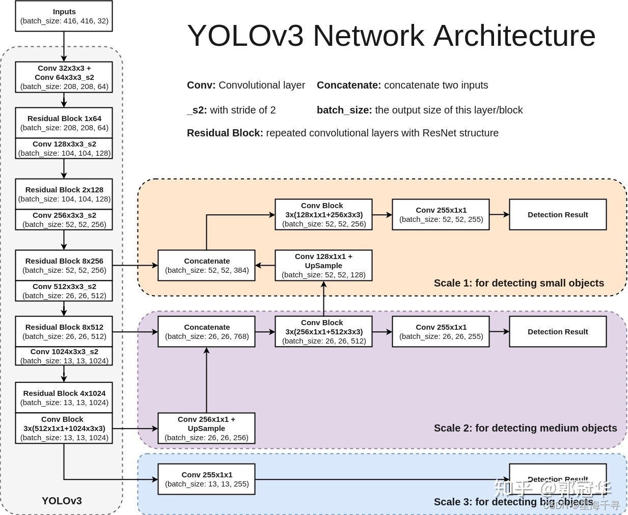
可以看出来，它有三个输出层，结果很多，定位也很详细。
参考自：https://zhuanlan.zhihu.com/p/40332004

2：COCO数据集 MS COCO的全称是Microsoft Common Objects in Context，起源于微软于2014年出资标注的Microsoft COCO数据集，与ImageNet竞赛一样，被视为是计算机视觉领域最受关注和最权威的比赛之一。 提供的类别有80 类，有超过33 万张图片，其中20 万张有标注，整个数据集中个体的数目超过150 万个。80个类别部分如下：

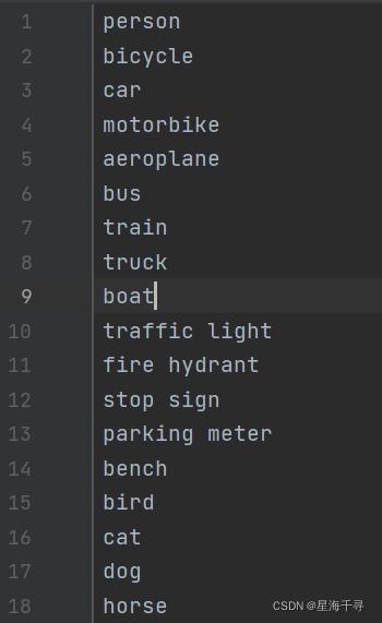
学习自：https://blog.csdn.net/qq_41185868/article/details/82939959

3：我们今天使用在coco数据集上训练好的yolov3模型，专门用于多物体的识别和定位。
下载地址：https://pjreddie.com/darknet/yolo/，今天我们不现场训练，而是使用现成的训练好的网络。

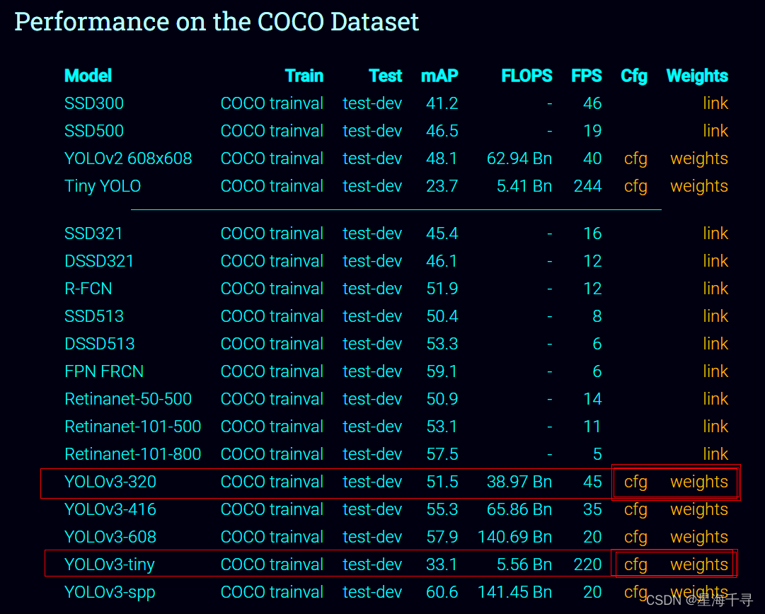
我们下载cfg文件（网络的架构）和weights文件（所有参数的权重）
我们可以看到yolov3-type，type越大，模型越大，输出结果越多，识别结果越精细，但是速度降低，FPS就越低了。相反type越小，模型越简单，输出结果越少， 识别结果越粗糙一点，但是速度提升了，FPS越高了。

点击后可以下载到本地。后续程序中要使用的。

4：opencv也是可以调用现成的深度神经网络模型的
可以调用，pytorch、tensorflow、darknet等深度学习模型。这里我们使用darknet的模型调用，其他的都是可以触类旁通的啊。
学习自：https://zhuanlan.zhihu.com/p/51928656
主要是学习主要的函数的使用。

第一部分：用一张图像测试

import cv2
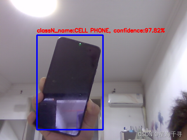
import numpy as npdef readAllCleassNames(filename):with open(filename, 'rt') as f:classNames = f.read().rstrip('\n').split('\n')return classNamesdef findAllObjects(outputs, img):confidence_threshold = 0.5h_src, w_src, c_src = img.shapeboundingbox = []  # 存储所有检结果的 boundingboxclassIds = []  # 存储所有检结果的 classnamecondiences = []  # 存储所有检结果的 confidence度，置信度for output in outputs:for result in output:head_confidence = result[4]  # 第五个值是总的置信度classes_confience = result[5:]  # 从第6个值开始到最后一共80个数值是每个class的置信度class_id = np.argmax(classes_confience)  # 获得哪个置信度最高就是认为是哪个classclass_max_confidence = classes_confience[class_id]  # 得到最高的置信度的数值# 进行置信度值过滤，confidence很低的就过滤掉if head_confidence > confidence_threshold and class_max_confidence > confidence_threshold:# 现在我们获得了一个结果cx, cy, w, h = result[0:4]  # 前俩个值是中心点的坐标，是算比例的，后俩数值是宽度和长度的比例# 将上述结果换算到原始图像上res_w, res_h = int(w_src * w), int(h_src * h)res_x, res_y = int(w_src * cx - 0.5 * res_w), int(h_src * cy - 0.5 * res_h)# 保存该结果boundingbox.append([res_x, res_y, res_w, res_h])classIds.append(class_id)condiences.append(class_max_confidence)# 进行NMS处理，这样经过非极大抑制后的结果更加准确，去掉了一些重复的区域。# 返回的结果indices是，保留了结果boundingbox的list下标。indices = cv2.dnn.NMSBoxes(boundingbox, condiences, confidence_threshold, nms_threshold=0.3)return boundingbox, classIds, condiences, indicesif __name__ == '__main__':# ======================= step 1: 先获得所有的类别信息classNames = readAllCleassNames('file/coco_classnames.txt')print(len(classNames))  # 一共有80个类别print(classNames)# ======================= step 2: 加载预先训练好的yolov3模型，加载模型和各个模型各个参数的权重值。# 这里加载的用DarkNet训练的模型和权重，还可以从Caffe, pytorch, tensor-flow, ONNX上加载对应的文件modelcfg = 'file/yolov3_320.cfg'modelWeights = 'file/yolov3_320.weights'# modelcfg = 'file/yolov3_tiny.cfg'# modelWeights = 'file/yolov3_tiny.weights'# 得到DarkNet上训练的yolov3模型和权重，得到了一个神经网络对象net = cv2.dnn.readNetFromDarknet(modelcfg, modelWeights)# 设置运行的背景，一般情况都是使用opencv dnn作为后台计算net.setPreferableBackend(cv2.dnn.DNN_BACKEND_OPENCV)# 设置目标设备, DNN_TARGET_CPU其中表示使用CPU计算，默认是的net.setPreferableTarget(cv2.dnn.DNN_TARGET_CPU)# ======================= step 3: 得到一个图像，转换后将其输入模型。img = cv2.imread('images/car_person.jpeg')# cv2.imshow('cat', img)# cv2.waitKey(0)# 转成blob的形式w_h_size = 320blob = cv2.dnn.blobFromImage(image=img,  # 输入图像scalefactor=1 / 255,  # 进行缩放，这个就是归一化操作，值全部在[0,1]之间size=(w_h_size, w_h_size),  # 输入图像的mean=[0, 0, 0],  # 给输入图像的每个通道的均值swapRB=1)  # 交换R和B通道net.setInput(blob)  # 设置输入# ======================= step 4: 得到输出结果，取出三个输出层的结果layerNames = net.getLayerNames()print(layerNames)  # 输入所有的每一层的名字和序号，这里返回layers的名字output_layers_ids = net.getUnconnectedOutLayers()  # yolov3有三个输出层print(output_layers_ids)  # 输入所有的输出层的序号，这里返回layers的下标序号，注意是从1开始的output_layers_names = [layerNames[layer_id - 1] for layer_id in output_layers_ids]print(output_layers_names)  # 得到所有的输出层的名字outputs = net.forward(output_layers_names)  # 设置前向传播的需要拿到的层的数据# print(len(outputs))  # 值是3， 因为yolov3有三个输出层# print(type(outputs))  # <class 'tuple'># 下面是yolov3-320的输出结果，它有三个输出层# print(type(outputs[0]))  # <class 'numpy.ndarray'># print(outputs[0].shape)  # (300, 85)，有300个结果，每个结果是(cx, cy, w, h, confidence, 80 * class_confidence)# print(type(outputs[1]))  # <class 'numpy.ndarray'># print(outputs[1].shape)  # (1200, 85)，有1200个结果，每个结果是(cx, cy, w, h, confidence, 80 * class_confidence)# print(type(outputs[2]))  # <class 'numpy.ndarray'># print(outputs[2].shape)  # (4800, 85)，有4800个结果，每个结果是(cx, cy, w, h, confidence, 80 * class_confidence)# 下面是yolov3-tiny的输出结果，yolov3-tiny只有两个输出层# print(type(outputs[0]))  # <class 'numpy.ndarray'># print(outputs[0].shape)  # (300, 85)，有300个结果，每个结果是(cx, cy, w, h, confidence, 80 * class_confidence)# print(type(outputs[1]))  # <class 'numpy.ndarray'># print(outputs[1].shape)  # (1200, 85)，有1200个结果，每个结果是(cx, cy, w, h, confidence, 80 * class_confidence)# ======================= step 5: 将结果解析，定在图上画出来bboxes, classids, confidences, indices = findAllObjects(outputs=outputs, img=img)print('In the end, we get {} results.'.format(len(indices)))  # 打印出我们得到了多少结果# 在原始图像上画出这个矩形框，以及在框上画出类别和置信度for idx in indices:bbox = bboxes[idx]class_name = classNames[classids[idx]]confidence = confidences[idx]x, y, w, h = bboxcv2.rectangle(img, pt1=(x, y), pt2=(x+w, y+h), color=(255, 0, 0), thickness=3)cv2.putText(img, text="classN_name:{}, confidence:{}%".format(class_name.upper(), "%.2f" % (confidence * 100)),org=(x, y-10), fontFace=cv2.FONT_HERSHEY_SIMPLEX, fontScale=0.6,color=(0, 0, 255), thickness=2)# 展示结果cv2.imshow('car_person', img)cv2.waitKey(0)

使用yolov3-320模型测试，准去度高，但是速度慢。

使用yolov3-tiny模型测试，准去度低很多，但是速度块很多。

第二部分：开启摄像头

import cv2
import numpy as npdef readAllCleassNames(filename):with open(filename, 'rt') as f:classNames = f.read().rstrip('\n').split('\n')return classNamesdef findAllObjects(outputs, img):confidence_threshold = 0.5h_src, w_src, c_src = img.shapeboundingbox = []  # 存储所有检结果的 boundingboxclassIds = []  # 存储所有检结果的 classnamecondiences = []  # 存储所有检结果的 confidence度，置信度for output in outputs:for result in output:head_confidence = result[4]  # 第五个值是总的置信度classes_confience = result[5:]  # 从第6个值开始到最后一共80个数值是每个class的置信度class_id = np.argmax(classes_confience)  # 获得哪个置信度最高就是认为是哪个classclass_max_confidence = classes_confience[class_id]  # 得到最高的置信度的数值# 进行置信度值过滤，confidence很低的就过滤掉if head_confidence > confidence_threshold and class_max_confidence > confidence_threshold:# 现在我们获得了一个结果cx, cy, w, h = result[0:4]  # 前俩个值是中心点的坐标，是算比例的，后俩数值是宽度和长度的比例# 将上述结果换算到原始图像上res_w, res_h = int(w_src * w), int(h_src * h)res_x, res_y = int(w_src * cx - 0.5 * res_w), int(h_src * cy - 0.5 * res_h)# 保存该结果boundingbox.append([res_x, res_y, res_w, res_h])classIds.append(class_id)condiences.append(class_max_confidence)# 进行NMS处理，这样经过非极大抑制后的结果更加准确，去掉了一些重复的区域。# 返回的结果indices是，保留了结果boundingbox的list下标。indices = cv2.dnn.NMSBoxes(boundingbox, condiences, confidence_threshold, nms_threshold=0.3)return boundingbox, classIds, condiences, indicesif __name__ == '__main__':# ======================= step 1: 先获得所有的类别信息classNames = readAllCleassNames('file/coco_classnames.txt')print(len(classNames))  # 一共有80个类别print(classNames)# ======================= step 2: 加载预先训练好的yolov3模型，加载模型和各个模型各个参数的权重值。# 这里加载的用DarkNet训练的模型和权重，还可以从Caffe, pytorch, tensor-flow, ONNX上加载对应的文件modelcfg = 'file/yolov3_320.cfg'modelWeights = 'file/yolov3_320.weights'# modelcfg = 'file/yolov3_tiny.cfg'# modelWeights = 'file/yolov3_tiny.weights'# 得到DarkNet上训练的yolov3模型和权重，得到了一个神经网络对象net = cv2.dnn.readNetFromDarknet(modelcfg, modelWeights)# 设置运行的背景，一般情况都是使用opencv dnn作为后台计算net.setPreferableBackend(cv2.dnn.DNN_BACKEND_OPENCV)# 设置目标设备, DNN_TARGET_CPU其中表示使用CPU计算，默认是的net.setPreferableTarget(cv2.dnn.DNN_TARGET_CPU)# ======================= step 3: 开启摄像头，得到一个图像，转换后将其输入模型。cap = cv2.VideoCapture(0)while True:ret, img = cap.read()if img is None:print("video is over...")break# 转成blob的形式w_h_size = 320blob = cv2.dnn.blobFromImage(image=img,  # 输入图像scalefactor=1 / 255,  # 进行缩放，这个就是归一化操作，值全部在[0,1]之间size=(w_h_size, w_h_size),  # 输入图像的mean=[0, 0, 0],  # 给输入图像的每个通道的均值swapRB=1)  # 交换R和B通道net.setInput(blob)  # 设置输入# ======================= step 4: 得到输出结果，取出三个输出层的结果layerNames = net.getLayerNames()# print(layerNames)  # 输入所有的每一层的名字和序号，这里返回layers的名字output_layers_ids = net.getUnconnectedOutLayers()  # yolov3有三个输出层# print(output_layers_ids)  # 输入所有的输出层的序号，这里返回layers的下标序号，注意是从1开始的output_layers_names = [layerNames[layer_id - 1] for layer_id in output_layers_ids]print(output_layers_names)  # 得到所有的输出层的名字outputs = net.forward(output_layers_names)  # 设置前向传播的需要拿到的层的数据# print(len(outputs))  # 值是3， 因为yolov3有三个输出层# print(type(outputs))  # <class 'tuple'># ======================= step 5: 将结果解析，定在图上画出来bboxes, classids, confidences, indices = findAllObjects(outputs=outputs, img=img)print('In the end, we get {} results.'.format(len(indices)))  # 打印出我们得到了多少结果# 在原始图像上画出这个矩形框，以及在框上画出类别和置信度for idx in indices:bbox = bboxes[idx]class_name = classNames[classids[idx]]confidence = confidences[idx]x, y, w, h = bboxcv2.rectangle(img, pt1=(x, y), pt2=(x+w, y+h), color=(255, 0, 0), thickness=3)cv2.putText(img, text="classN_name:{}, confidence:{}%".format(class_name.upper(), "%.2f" % (confidence * 100)),org=(x, y-10), fontFace=cv2.FONT_HERSHEY_SIMPLEX, fontScale=0.6,color=(0, 0, 255), thickness=2)# 展示结果cv2.imshow('test', img)cv2.waitKey(1)

效果如下：